Training Metrics

We use several metrics to evaluate the performance of your machine learning model. These metrics are categorized into three groups:

• Performance-focused metrics: Used to select the best cycle for a single experiment.
• Sustainability-focused metrics: Measure the environmental impact of training.
• Mixed metrics: Combine both performance and sustainability factors to compare multiple experiments.

1. Performance-focused metrics

We use the following example to demonstrate the calculation of these metrics:

ground_truth = [1, 1, 1, 0, 0, 1, 0, 1, 0]
prediction = [1, 1, 0, 0, 1, 1, 0, 1, 0]

There are four different outcomes for the models prediction:

def true_positive(ground_truth, prediction):
    tp = 0
    for gt, pred in zip(ground_truth, prediction):
        if gt == 1 and pred == 1:
            tp +=1
    return tp

def true_negative(ground_truth, prediction):
    tn = 0
    for gt, pred in zip(ground_truth, prediction):
        if gt == 0 and pred == 0:
            tn +=1
    return tn

def false_positive(ground_truth, prediction):
    fp = 0
    for gt, pred in zip(ground_truth, prediction):
        if gt == 0 and pred == 1:
            fp +=1
    return fp

def false_negative(ground_truth, prediction):
    fn = 0
    for gt, pred in zip(ground_truth, prediction):
        if gt == 1 and pred == 0:
            fn +=1
    return fn

For our example we have:

true_positive(ground_truth, prediction)
# out: 4
true_negative(ground_truth, prediction)
# out: 3
false_positive(ground_truth, prediction)
# out: 1
false_negative(ground_truth, prediction)
# out: 1

Here are the main metrics that fall in this criteria:

Accuracy

The accuracy is a measure of how well a model correctly predicts the output for a given input. It is calculated by dividing the number of correct predictions by the total number of predictions made.

def accuracy(ground_truth, prediction):
    tp = true_positive(ground_truth, prediction)  
    fp = false_positive(ground_truth, prediction)
    tn = true_negative(ground_truth, prediction)
    fn = false_negative(ground_truth, prediction)
    accuracy = (tp + tn) / (tp + fp + tn + fn)
    return accuracy

# Example:

accuracy(ground_truth, prediction)
# out: 7/9 

Loss

Loss quantifies how far off a model’s predictions are from the true values. Lower loss indicates better performance.

Precision

Precision is a measure of the number of correct positive predictions made by the model, compared to the total number of positive predictions made. In other words, the precision of a model shows how accurate the positive predictions are.

def precision(ground_truth, prediction):
    tp = true_positive(ground_truth, prediction)  
    fp = false_positive(ground_truth, prediction)  
    prec = tp / (tp + fp)  
    return prec

# Example

precision(ground_truth, prediction)
# out: 0.8

Recall

Recall is a measure of the number of correct positive predictions made by the model, compared to the total number of actual positive instances. In other words, the recall (also called "sensitivity") of the model shows the coverage of actual positive samples.

def recall(ground_truth, prediction):
    tp = true_positive(ground_truth, prediction)  
    fp = false_positive(ground_truth, prediction)  
    rec = tp / (tp + fn)  
    return rec

# Example

recall(ground_truth, prediction)
# out: 0.8

F1-score

The F1-score is the harmonic mean of precision and recall. It is a good metric to use when you want to balance precision and recall.

def f1(ground_truth, prediction):
    p = precision(ground_truth, prediction)
    r = recall(ground_truth, prediction)
    f1_score = 2 * p * r/ (p + r) 
    return f1_score

# Example

f1_score(ground_truth, prediction)
# out: 0.8

Mean Average Precision (mAP)

Mean Average Precision (mAP) is a common metric used in evaluating the performance of object detection models. It calculates the average precision (AP) for each class and then averages these values. It takes into account both precision and recall over different thresholds.

def average_precision(precision, recall):
    precision = np.array(precision)
    recall = np.array(recall)
    ap = np.sum((recall[1:] - recall[:-1]) * precision[1:])
    return ap

def mean_average_precision(ground_truths, predictions):
    aps = []
    for i in range(len(ground_truths)):
        precision = precision(ground_truths[i], predictions[i])
        recall = recall(ground_truths[i], predictions[i])
        ap = average_precision(precision, recall)
        aps.append(ap)
    return np.mean(aps)

# Example

mean_average_precision(ground_truth, prediction)
# out: 0.75

Intersection over Union (IoU)

Intersection over Union (IoU) is a metric used to evaluate the accuracy of an object detector on a particular dataset. It is calculated as the area of the intersection divided by the area of the union of the predicted and ground truth bounding boxes.

def iou(ground_truth, prediction):
    x1 = max(ground_truth[0], prediction[0])
    y1 = max(ground_truth[1], prediction[1])
    x2 = min(ground_truth[2], prediction[2])
    y2 = min(ground_truth[3], prediction[3])

    intersection = max(0, x2 - x1) * max(0, y2 - y1)
    gt_area = (ground_truth[2] - ground_truth[0]) * (ground_truth[3] - ground_truth[1])
    pred_area = (prediction[2] - prediction[0]) * (prediction[3] - prediction[1])
    union = gt_area + pred_area - intersection

    iou_score = intersection / union
    return iou_score

# Example

iou(ground_truth, prediction)
# out: 0.67

Mean Absolute Error (MAE)

Mean Absolute Error (MAE) measures the average magnitude of errors in a set of predictions, without considering their direction. It's the average over the test sample of the absolute differences between prediction and actual observation where all individual differences have equal weight.

def mae(ground_truth, prediction):
    error = np.abs(ground_truth - prediction)
    return np.mean(error)

# Example

mae(ground_truth, prediction)
# out: 3.2

Percentage of Correct Keypoints (PCK)

Percentage of Correct Keypoints (PCK) is a metric used to evaluate the accuracy of predicted keypoints, commonly used in human pose estimation. A keypoint is considered correct if its distance from the ground truth is within a certain threshold, usually defined as a fraction of a predefined reference length (like the torso length).

def pck(ground_truth_keypoints, predicted_keypoints, threshold=0.2):
    correct_keypoints = 0
    total_keypoints = len(ground_truth_keypoints)
    
    for gt, pred in zip(ground_truth_keypoints, predicted_keypoints):
        distance = np.linalg.norm(np.array(gt) - np.array(pred))
        reference_length = np.linalg.norm(np.array(ground_truth_keypoints[1]) - np.array(ground_truth_keypoints[2]))  # Example: distance between two keypoints like shoulder and hip
        if distance / reference_length <= threshold:
            correct_keypoints += 1
            
    pck_score = correct_keypoints / total_keypoints
    return pck_score

# Example

ground_truth_keypoints = [(10, 20), (30, 40), (50, 60), (70, 80)]  # Example keypoints
predicted_keypoints = [(12, 22), (33, 45), (47, 62), (69, 79)]  # Example predictions
pck(ground_truth_keypoints, predicted_keypoints, threshold=0.2)
# out: 0.75

Vgap

Vgap is a metric that measures the absolute difference between the validation loss and the training loss. A larger vgap indicates that the model may be overfitting the training data.

def vgap(training_loss, validation_loss):
    vgap = abs(training_loss - validation_loss)
    return vgap

Flops

Flops, or floating point operations, are a measure of the computational power of a model. A model with a higher flops value required more computational resources to run.

2. Sustainability-focused metrics

gCO2e

gCO2e stands for "grams carbon dioxide equivalent." It is a measure of the environmental impact of training a machine learning model, up to a certain point in the training process.

gCO2e compares emissions from different greenhouse gases based on their global warming potential (GWP). It converts the amount of other gases into the equivalent amount of CO2 in grams.

For example, methane has a GWP of 25, meaning that the emission of one gram of methane is equivalent to the emission of 25 grams of carbon. Carbon is used as a reference and has a GWP of 1.

Calculation

To calculate gCO2e, we estimate the energy consumption of the GPU by looking at the training time and utilization rate. We then use the carbon intensity (gCO2e/kWh) of the computation center to calculate the gCO2e.

3. Mixed Metrics

The mixed metrics are benchmarks that take into account two or more of the previously discussed metrics in order to find the best experiment from a group of experiments.

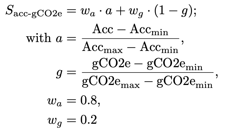
acc-gCO2e

Weighted sum of training accuracy and normalized gCO2e emission. The accuracy to gCO2e weight ratio is 80/20. The gCO2e emission is normalized over all experiments on a dataset by min-max scaling the gCO2e value to the interval [0,1]. A score of 1 marks the best performance.

Equations

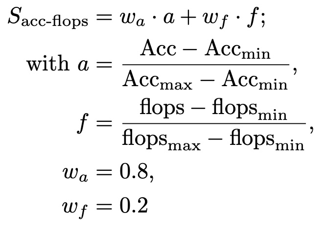
acc-flops

Weighted sum of training accuracy and normalized flops. The accuracy to flops weight ratio is 80/20. The flops are normalized over all experiments on a dataset by min-max scaling the flops value to the interval [0,1]. A score of 1 marks the best performance.

Equations

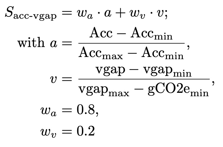
acc-vgap

Weighted sum of training accuracy and normalized vgap. The accuracy to vgap weight ratio is 80/20. The vgap is normalized over all experiments on a dataset by min-max scaling the vgap value to the interval [0,1]. A score of 1 marks the best performance.

Equations

pck-gCO2e

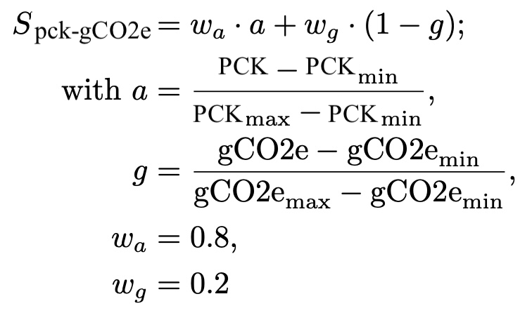
Weighted sum of training pck and normalized gCO2e emission. The pck to gCO2e weight ratio is 80/20. The gCO2e emission is normalized over all experiments on a dataset by min-max scaling the gCO2e value to the interval [0,1]. A score of 1 marks the best performance.

Equations

pck-flops

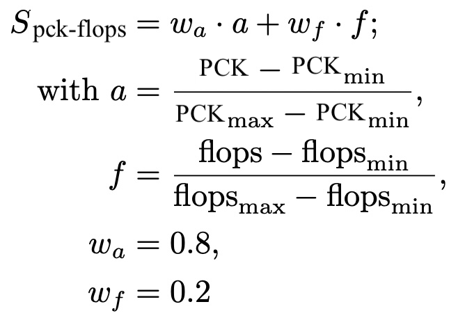
Weighted sum of training pck and normalized flops. The pck to flops weight ratio is 80/20. The flops are normalized over all experiments on a dataset by min-max scaling the flops value to the interval [0,1]. A score of 1 marks the best performance.

Equations

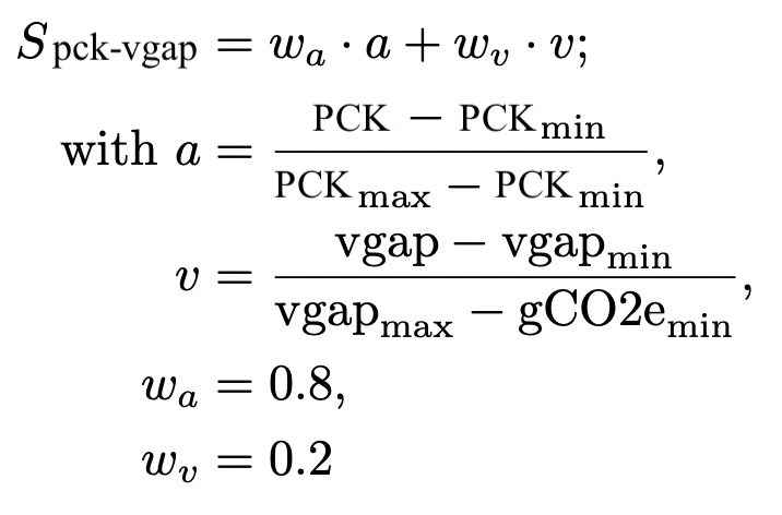
pck-vgap

Weighted sum of training pck and normalized vgap. The pck to vgap weight ratio is 80/20. The vgap is normalized over all experiments on a dataset by min-max scaling the vgap value to the interval [0,1]. A score of 1 marks the best performance.

Equations